: Boundary conditions at interfaces
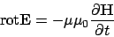
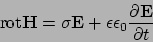
: Maxwell Equation
: Energy Conservation
From Eq.3 and Eq.6
 |
(13) |
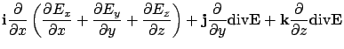
From Eqs.4, 5, 7
 |
(14) |
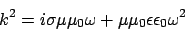
If we apply  to Eq.13 and
 to Eq.14
and using the relation
to Eq.14
and using the relation
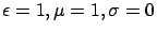
If we assume  ,
,
 then
then
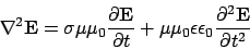 |
(16) |
In the same way we can get
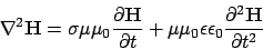 |
(17) |
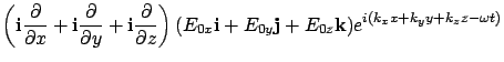
In the case that the electric field is plane wave
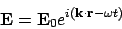 |
(18) |
then
 |
(19) |
In vacuum,
 and
and
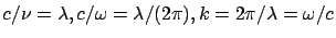 then
then
 |
(20) |
If we define the comlex optical index  by
by
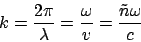 |
(21) |
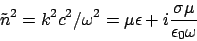 |
(22) |
1
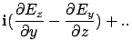
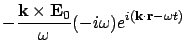
If we take divergence of electic filed in the form of plane wave.
Then the electric field is transverse wave.
If the magnetic-flux density  is written as
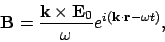 |
(31) |
the magnetic-flux density satisfies Eq.3, because
In vacuum
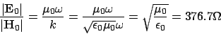 |
(37) |
: Boundary conditions at interfaces
: Maxwell Equation
: Energy Conservation
Yamamoto Masahiro
�$BJ?@.�(B14�$BG/�(B8�$B7n�(B30�$BF|�(B
![$\displaystyle {\bf i} \left[ \frac{\partial^2 E_y}{\partial x \partial y} -
\fr...
...frac{\partial ^2 E_z}{\partial x \partial z}\right] + {\bf j}[..] + {\bf k}[..]$](img63.png)